两个频谱范围比较接近的信号如何分离？

乔帮主

比如一个能量主要分布在300-1000，另一个在600-1500，这种信号该如何做到分离呢

原文地址：https://www.zhihu.com/question/455796872

检验医师

这大部分模态分解方法和盲源分离方法都将失效，试试Void-Kalman滤波方法吧，也不一定能成功
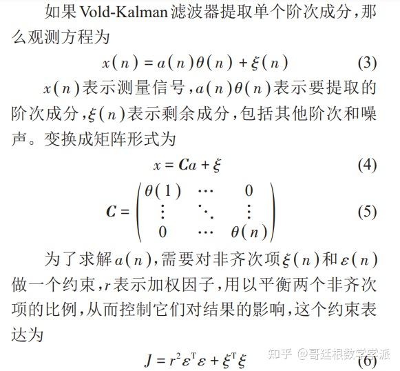
1993 年, VOLD 和 LEURIDAN 以现代控制理论中的卡尔曼滤波原理为理论基础, 提出了 Vold -Kalman 跟踪滤波方法, 开创了在时域中直接提取阶比分量的先河，Vold-Kalman阶次追踪可以提取多个阶次分量，其解耦临近和交叉阶次的准确性也较好，在很多领域得到了广泛应用。




         为了追踪目标阶次的信号，构建状态方程和观测方程，信号模型用幅值和载波乘积的形式表达，通过求得的包络幅值重构阶次信号。将阶次信号模型表示为幅值和载波的乘积：






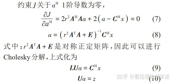
先通过向前分解求出z，再通过向后代入求a，由此完成对包含多重分量复杂信号的阶比分量提取。提取出的单个阶比的信号往往可以对应到分析场中的局部特征，通过对阶比信号追踪分析，就可对信号的各个子特征进行识别。
首先导入相关模块
import numpy as np
from scipy import sparse
from scipy.linalg import pascal
from scipy.sparse import linalg
import matplotlib.pyplot as plt
import time定义Void-Kalman函数
def vkf(y,fs,f,p=None,bw=None,multiorder=None,solver='scipy-spsolve'):
    """
    参数
    ----------
    y : 输入信号
    fs :采样频率
    f : 信号y的频率序列[f_1,...,f_K]
    p : p 阶滤波器（通常在 1 或 4 之间）
    bw : 带宽，默认为bw=fs/100
    multiorder : 算法的阶数
    solver : 'scikits-spsolve' (faster) or 'scipy-spsolve' (slower)
    返回值
    -------
    x : 复包络
    c : 相位  
    """
   
    if type(p)==type(None):
        p = 2#Default filter order
    if type(bw) ==type(None):
        bw = fs/100   #Default bandwidth: 0.01*fs
    if type(multiorder)==type(None):
        multiord = True   #Default single-order algorithm
    else:
        multiord = multiorder
    silent=False

    if len(np.array(y).shape)>1:
        if np.array(y).shape[1] > np.array(y).shape[0]:   
            y = np.transpose(np.array(y))
    else:
        y = np.array(y)
    if np.size(bw)!=1:   
        if np.array(bw).shape[1] > np.array(bw).shape[0]:
            bw = np.transpose(np.array(bw))
        else:
            bw = np.array(bw)
    if silent ==False:
        print('preparing array ok')
    #Signal
    n_t = len(y)
   
    #频率向量
    (n_f, n_ord) = f.shape
    if n_f == 1:
        f1 = np.ones(n_t,1)*f
        raise Warning('error:', f1)
    elif n_f != n_t:
        raise Warning('The array in f should have 1 or {} elements.'.format(n_t))
   
    #将频率向量转换为相位向量
    c = np.exp(2j*np.pi*np.cumsum(f,axis=0)/fs)
    #带宽向量
    n_bw = np.size(bw)
    if n_bw == 1:
        bw = np.ones((n_t,1))*bw
    elif n_bw != n_t:
        raise Warning('The array bw should have 1 or {} elements.'.format(n_t))
   
    #以弧度为单位的相对带宽
    phi = np.pi/fs*bw
    #滤波器阶数
    p_tmp = p
    if np.size(p)>1:
        p = max(p)
    p_lo = np.setdiff1d(p_tmp,p)
     
    #构造滤波器矩阵和带宽向量
    P_lu = pascal(p+1,kind='lower',exact=True)
    signalt = np.empty((p+1,))
    signalt[::2] = 1
    signalt[1::2] = -1
    coeffs = P_lu[-1,:]*signalt

    #差分方程的线性系统
    A = sparse.spdiags((np.ones((n_t,1))*coeffs).transpose(),np.arange(0,p+1),n_t-p,n_t)

    #引入低阶方程以将边界条件设置为零
    pp = np.size(p_lo)
    A_pre = sparse.csr_matrix((pp,n_t), dtype=None) #sparse(pp,n_t)
    A_pre[:,0:p+1] = P_lu[p_lo,0:p+1]
    A = sparse.vstack([A_pre, A, A_pre[-1::-1,-1::-1]])
   
   
    s = np.arange(0,p+1)
    sgn = np.power(-1,s)
   
    Q = np.zeros((p+1,p+1))
    b = np.zeros((p+1,1))
   
    Q[0,:] = np.ones((p+1))
    b[0] = 2**(2*p-1)
   
    for i in range(0,p):
        Q[i+1,:] = np.power(s,(2*(i))) * sgn
   
    q = np.linalg.solve(Q,b).transpose()*sgn

    num = np.sqrt(2)-1
    den = np.zeros((np.size(bw),1))
    for qi in range(0,np.size(q)):
        den = den + 2*q[0,qi]*np.cos((qi)*phi)
    r = np.sqrt(num/den)


    if (den <= 0).any() | (r > (np.sqrt(1/(2*q[0,0]*np.finfo(float).eps)))).any():
        raise Warning('Ill-conditioned B-matrix selectivity bandwidth is too small.')

    R = sparse.spdiags(r.transpose(),0,n_t,n_t)
    B = (A.dot(R)).transpose().dot(A.dot(R)) + sparse.eye(n_t)

    del A, A_pre, R, bw, phi, num, den, f
   
   
    if multiord:
        nn = n_t*n_ord
        diags = list(range(-p,p+1))
        diags_B = np.zeros((B.shape[0],len(diags)))
        for i in range(0,len(diags)):
            if diags==0:
                diags_B[:,i] = B.diagonal(diags)
            elif diags>0:
                diags_B[:-diags,i] = B.diagonal(diags)
            elif diags<0:
                diags_B[:diags,i] = B.diagonal(diags)
        diags_B_r= np.tile(diags_B.T,(1,n_ord))

        BB_D = sparse.diags(diags_B_r,diags,shape=(nn,nn))

        bl_U = int((n_ord**2 - n_ord)/2)

        ii_U = np.zeros((n_t,bl_U))
        jj_U = np.zeros((n_t,bl_U))
        cc_U = np.zeros((n_t,bl_U),dtype = np.float64)
        m = 0
        
        for ki in range(0,n_ord):
            for kj in range((ki+1),n_ord):
                ii_U[:,m] = (ki)*n_t + np.arange(0,n_t)
                jj_U[:,m] = (kj)*n_t + np.arange(0,n_t)
                cc_U[:,m] = np.real(np.conj(c[:,ki])*c[:,kj])
                m = m + 1

        BB_U = sparse.csr_matrix((cc_U.flatten(),(ii_U.flatten(),jj_U.flatten())),shape=(nn,nn))
        
        BB = BB_D + BB_U + BB_U.transpose()

        cy = (np.conj(c.T.reshape(-1,1)).T*np.tile(y,(n_ord))).T

        del diags_B, B, BB_D, BB_U, ii_U, jj_U, cc_U   
   
   
    if silent==False:
        print('Solving sparse Ax=b, as single precision complex')
    if multiord:
        if solver=='scikits-spsolve':
            from scikits import umfpack
            xx = 2 * umfpack.spsolve(BB,cy)
        else:
            xx = linalg.spsolve(BB,cy,use_umfpack=False)
        # xx = bicg(BB,cy)
        x = 2 * xx.reshape(n_ord,-1).T  
    else:
        x = np.zeros((n_t,n_ord),dtype=np.complex64)
        for ki in range(0,n_ord):
            cy_k = np.conj(c[:,ki])*y
            if solver=='scikits-spsolve':
                from scikits import umfpack
                x[:,ki] = 2 * umfpack.spsolve(B,cy_k)
            else:
                print('dtype B: ',B.dtype)
                # x[:,ki] = 2 * linalg.lgmres(B,cy_k)
                x[:,ki] = 2 * linalg.spsolve(B,cy_k,use_umfpack=False)
   
    return x,c,r

def lil_repeat(S, repeat):
   
    shape=list(S.shape)
    if isinstance(repeat, int):
        shape[0]=shape[0]*repeat
    else:
        shape[0]=sum(repeat)
    shape = tuple(shape)
    new = sparse.lil_matrix(shape, dtype=S.dtype)
    new.data = S.data.repeat(repeat) # flat repeat
    new.rows = S.indices.repeat(repeat)
    return new下面进行验证，首先设置一些基本参数，例如采样频率，时间项等
fs = 12000
T = 50
dt = 1/fs
t = np.linspace(0,(T),np.int64((T-dt)/dt+1)).transpose()
N = t.size然后构造第1个非平稳成分
A0 = 2*np.hstack([np.linspace(0.5,1,np.floor(N/2).astype(np.int64())), np.linspace(1,0.5,np.ceil(N/2).astype(np.int64()))])
f0 = (0.2*fs - 0.1*fs*np.cos(4*np.pi*t/T)).reshape(-1,1)
phi0 = 2*np.pi*np.cumsum(f0)*dt+3*t/max(t)
y0 = A0*np.cos(phi0)构造第2个非平稳成分
A1 = np.hstack([np.linspace(0.5,1,np.floor(N/2).astype(np.int64())), np.linspace(1,0.5,np.ceil(N/2).astype(np.int64()))])
f1 = (0.2*fs - 0.1*fs*np.cos(np.pi*t/T)).reshape(-1,1)
phi1 = 2*np.pi*np.cumsum(f1)*dt
y1 = A1*np.cos(phi1)构造第3个非平稳成分
As1 = np.ones(N)
fs1 = 0.2*fs*np.ones((N,1))
phis1 = 2*np.pi*np.cumsum(fs1)*dt
ys1 = As1*np.sin(phis1)加点白噪声干扰
    e = 1.5*np.random.rand(np.size(y1))构造试验用复合信号
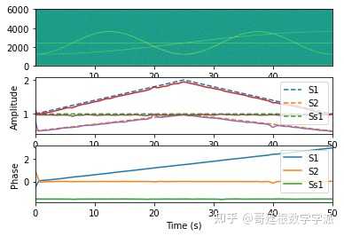
    y = y0+ y1 + ys1 + e执行Void-Kalman滤波
p = 2
bw = fs/12000
t1=time.time()
(x,c,r) = vkf(y,fs,np.hstack([f0, f1, fs1]),p=p,bw=bw)
print('elaspsed time: {}'.format(time.time()-t1))
xreal = np.real(x*c)显示白噪声
w = y-np.sum(xreal,1)幅值与相位
Amplitude = np.abs(x)
Phase = np.log(x).imag作图
fig,ax = plt.subplots(nrows=3)
ax[0].specgram(y,round(fs/16),Fs=fs)
ax[1].plot(t,np.vstack((A0,A1,As1)).T,'--')
ax[1].plot(t,Amplitude)
ax[1].set_xlim([min(t),max(t)])
ax[2].plot(t,Phase)
ax[2].set_xlim([min(t),max(t)])
ax[2].set_xlabel('Time (s)')
ax[1].set_ylabel('Amplitude')
ax[2].set_ylabel('Phase')
ax[1].legend(['S1','S2','Ss1'],loc='upper right')
ax[2].legend(['S1','S2','Ss1'],loc='upper right')
  

大力水手

这都相互干扰了，没法分离。这种频谱重叠的干扰跟混叠一样啊不可逆的，频域上没法处理。必须要分开才行。如果强行加滤波器可以减少另一个的干扰强度，但是没法消除